GWDataNoiseSource Tutorial

The GWDataNoiseSource is a data source element that generates realistic gravitational wave detector noise with an appropriate power spectral density (PSD). This tutorial will guide you through generating, analyzing, and visualizing simulated gravitational wave strain data.

Overview

LIGO (Laser Interferometer Gravitational-Wave Observatory) and Virgo are gravitational wave detectors that measure tiny distortions in spacetime caused by passing gravitational waves. The background noise in these detectors has specific spectral characteristics.

The GWDataNoiseSource produces simulated strain data with noise characteristics inspired by modern GW detectors, useful for:

• Testing data analysis pipelines
• Developing and validating gravitational wave search algorithms
• Educational demonstrations
• Software validation

Step 1: Generate Simulated Strain Data

Let's create a script that generates simulated gravitational wave detector noise for multiple detectors:

#!/usr/bin/env python3
"""
Generate simulated LIGO/Virgo gravitational wave detector noise.

This script creates a pipeline with GWDataNoiseSource to generate strain
data for specified detectors and writes the output to text files.
"""

import os
import argparse
from sgn.apps import Pipeline
from sgnts.sinks import DumpSeriesSink
from sgnligo.sources.gwdata_noise_source import GWDataNoiseSource


def main():
    # Parse command line arguments
    parser = argparse.ArgumentParser(description="Generate gravitational wave detector noise")
    parser.add_argument("--duration", type=float, default=50.0,
                      help="Duration in seconds (default: 50.0)")
    parser.add_argument("--detectors", type=str, default="H1,L1",
                      help="Comma-separated list of detectors (default: 'H1,L1')")
    parser.add_argument("--output-dir", type=str, default="./strain_output",
                      help="Directory to save output files (default: ./strain_output)")
    parser.add_argument("--real-time", action="store_true",
                      help="Generate data in real time")
    parser.add_argument("--verbose", action="store_true",
                      help="Print verbose output")
    args = parser.parse_args()

    # Create output directory
    os.makedirs(args.output_dir, exist_ok=True)

    # Parse detectors
    detectors = [d.strip() for d in args.detectors.split(",")]

    # Create channel dictionary
    channel_dict = {detector: f"{detector}:FAKE-STRAIN" for detector in detectors}

    # Set up pipeline
    pipe = Pipeline()

    # Create noise source
    source = GWDataNoiseSource(
        name="NoiseSource",
        channel_dict=channel_dict,
        duration=args.duration,
        real_time=args.real_time,
        verbose=args.verbose
    )

    # Create sinks for each channel
    sinks = {}
    for detector, channel_name in channel_dict.items():
        output_file = os.path.join(args.output_dir, f"{detector}_strain.txt")
        sinks[detector] = DumpSeriesSink(
            name=f"Sink_{detector}",
            sink_pad_names=[channel_name],
            fname=output_file,
            verbose=args.verbose
        )

    # Add source and sinks to pipeline
    elements = [source] + list(sinks.values())
    pipe.insert(*elements)

    # Create link map
    link_map = {}
    for detector, channel_name in channel_dict.items():
        link_map[f"Sink_{detector}:snk:{channel_name}"] = f"NoiseSource:src:{channel_name}"

    # Add connections to pipeline
    pipe.insert(link_map=link_map)

    # Run the pipeline
    print(f"Generating {args.duration} seconds of strain data for detectors: {detectors}")
    pipe.run()
    print("Pipeline completed successfully")
    print(f"Output files written to {args.output_dir}")


if __name__ == "__main__":
    main()

Save this script as generate_strain.py. You can run it with various options:

# Generate 50 seconds of data for LIGO Hanford (H1) and Livingston (L1)
python generate_strain.py

# Generate 30 seconds of data for all three detectors (H1, L1, V1)
python generate_strain.py --duration 30.0 --detectors H1,L1,V1 

The script will create text files containing the simulated strain data, one file per detector.

Step 2: Analyze and Visualize the Data

Now let's create a script to analyze and visualize the simulated strain data:

#!/usr/bin/env python3
"""
Analyze and visualize simulated gravitational wave detector strain data.

This script reads strain data files, calculates spectral properties,
and creates visualizations including time series, PSDs, and spectrograms.
"""

import os
import argparse
import glob
import numpy as np
import matplotlib.pyplot as plt
from scipy import signal


def read_strain_file(filename):
    """Read strain data from a text file."""
    # Load data, skipping any comment lines
    data = np.loadtxt(filename, comments='#')

    # Extract time and strain
    times = data[:, 0]
    strain = data[:, 1]

    # Get detector from filename
    detector = os.path.basename(filename).split("_")[0]

    return times, strain, detector


def plot_strain_timeseries(times, strain, detector, output_dir):
    """Plot the strain time series data."""
    # Make times relative to start
    rel_times = times - times[0]

    plt.figure(figsize=(12, 6))

    # Plot time series
    plt.plot(rel_times, strain, 'k-', linewidth=0.5)
    plt.title(f"{detector} Strain Data Time Series")
    plt.xlabel("Time (s)")
    plt.ylabel("Strain")
    plt.grid(True, alpha=0.3)

    # Save figure
    os.makedirs(output_dir, exist_ok=True)
    plt.savefig(os.path.join(output_dir, f"{detector}_timeseries.png"), dpi=300)
    plt.close()


def plot_strain_asd(strain, detector, output_dir, sample_rate=16384):
    """Calculate and plot the amplitude spectral density."""
    # Calculate PSD using Welch's method
    f, Pxx = signal.welch(strain, fs=sample_rate, nperseg=4096, noverlap=2048)

    # Calculate ASD (amplitude spectral density)
    asd = np.sqrt(Pxx)

    plt.figure(figsize=(12, 6))

    # Plot ASD
    plt.loglog(f, asd)
    plt.title(f"{detector} Amplitude Spectral Density")
    plt.xlabel("Frequency (Hz)")
    plt.ylabel("Strain/√Hz")
    plt.xlim([10, sample_rate/2])
    plt.grid(True, which="both", alpha=0.3)

    # Save figure
    os.makedirs(output_dir, exist_ok=True)
    plt.savefig(os.path.join(output_dir, f"{detector}_asd.png"), dpi=300)
    plt.close()


def plot_strain_spectrogram(strain, detector, output_dir, sample_rate=16384):
    """Create a spectrogram visualization."""
    # Calculate spectrogram
    f, t, Sxx = signal.spectrogram(strain, fs=sample_rate, nperseg=1024, noverlap=900)

    plt.figure(figsize=(12, 6))

    # Plot spectrogram
    plt.pcolormesh(t, f, 10 * np.log10(Sxx), shading='gouraud')
    plt.title(f"{detector} Strain Spectrogram")
    plt.ylabel("Frequency (Hz)")
    plt.xlabel("Time (s)")
    plt.colorbar(label="PSD [dB/Hz]")
    plt.yscale("log")
    plt.ylim([20, sample_rate/2])

    # Save figure
    os.makedirs(output_dir, exist_ok=True)
    plt.savefig(os.path.join(output_dir, f"{detector}_spectrogram.png"), dpi=300)
    plt.close()


def create_detector_comparison(strain_files, output_dir, sample_rate=16384):
    """Create a comparison of ASDs from all detectors."""
    plt.figure(figsize=(12, 8))

    # Colors for each detector
    colors = {"H1": "r", "L1": "b", "V1": "g"}
    labels = {"H1": "LIGO Hanford", "L1": "LIGO Livingston", "V1": "Virgo"}

    for file in strain_files:
        times, strain, detector = read_strain_file(file)

        # Calculate ASD
        f, Pxx = signal.welch(strain, fs=sample_rate, nperseg=4096, noverlap=2048)
        asd = np.sqrt(Pxx)

        # Plot with detector-specific color and label
        color = colors.get(detector, "k")
        label = labels.get(detector, detector)
        plt.loglog(f, asd, color=color, label=label, alpha=0.8)

    plt.title("Detector Sensitivity Comparison")
    plt.xlabel("Frequency (Hz)")
    plt.ylabel("Strain/√Hz")
    plt.xlim([10, sample_rate/2])
    plt.grid(True, which="both", alpha=0.3)
    plt.legend()

    # Save figure
    os.makedirs(output_dir, exist_ok=True)
    plt.savefig(os.path.join(output_dir, "detector_comparison.png"), dpi=300)
    plt.close()


def main():
    parser = argparse.ArgumentParser(description="Analyze and plot strain data")
    parser.add_argument("--input-dir", type=str, default="./strain_output",
                      help="Directory containing strain files (default: ./strain_output)")
    parser.add_argument("--output-dir", type=str, default="./plots",
                      help="Directory to save plots (default: ./plots)")
    args = parser.parse_args()

    # Find all strain data files
    strain_files = sorted(glob.glob(os.path.join(args.input_dir, "*_strain.txt")))

    if not strain_files:
        print(f"No strain data files found in {args.input_dir}")
        return

    print(f"Found {len(strain_files)} strain data files")

    # Create output directory
    os.makedirs(args.output_dir, exist_ok=True)

    # Process each file
    for file in strain_files:
        print(f"Processing {file}")
        times, strain, detector = read_strain_file(file)

        # Create plots
        plot_strain_timeseries(times, strain, detector, args.output_dir)
        plot_strain_asd(strain, detector, args.output_dir)
        plot_strain_spectrogram(strain, detector, args.output_dir)

    # Create comparison plot
    if len(strain_files) > 1:
        create_detector_comparison(strain_files, args.output_dir)

    print(f"Plots saved to {args.output_dir}")


if __name__ == "__main__":
    main()

Save this script as analyze_strain.py. You can run it after generating strain data:

# Analyze and plot strain data
python analyze_strain.py --input-dir ./strain_output --output-dir ./plots

Example Output

Here's an example of what the generated strain plots should look like:

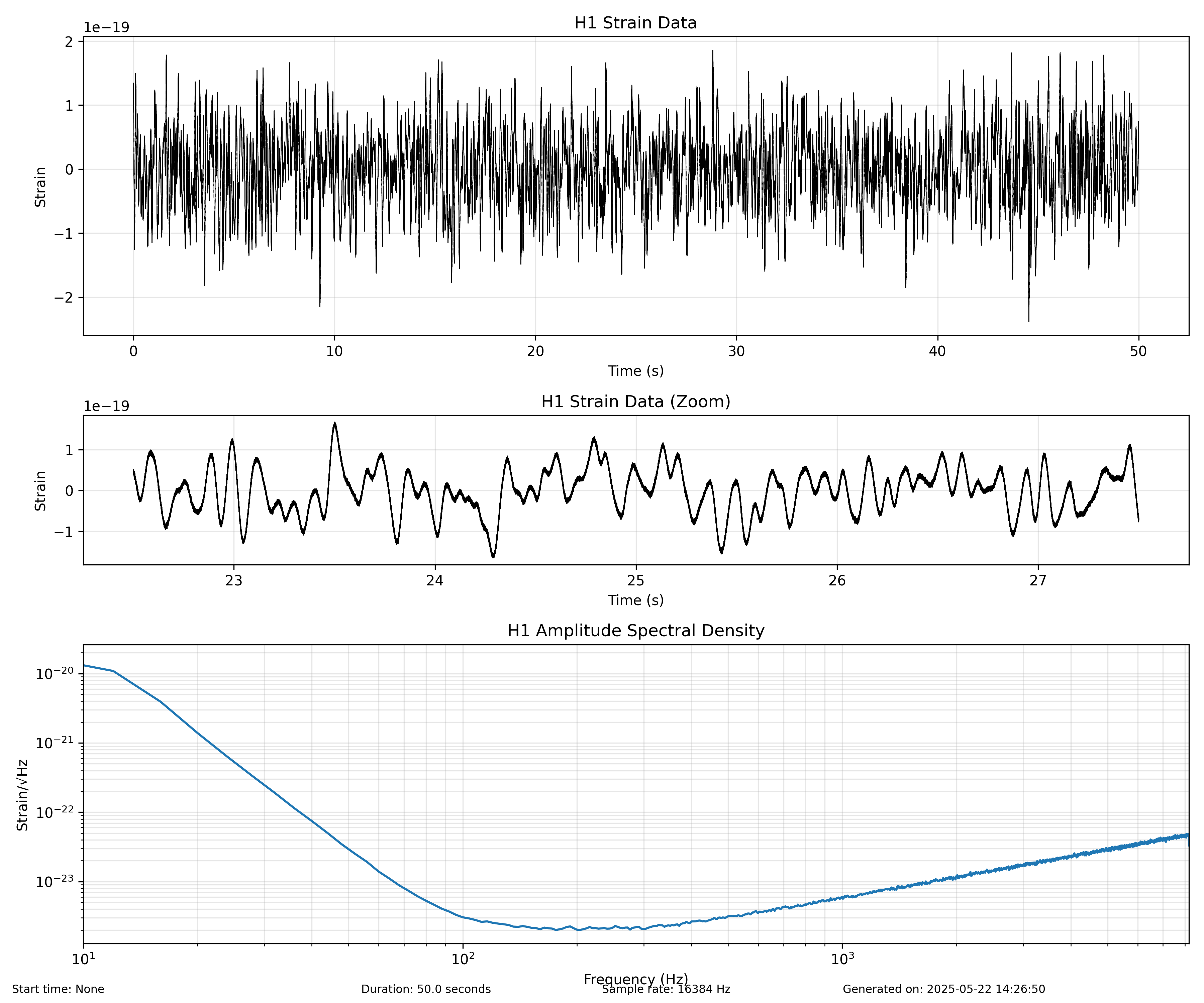
Figure: Example H1 strain data time series showing realistic gravitational wave detector noise with characteristic spectral properties.

GWDataNoiseSource Details

The GWDataNoiseSource has the following important parameters:

Key Parameters

• name: Element name used in the pipeline
• channel_dict: Dictionary mapping detector names to channel names
• t0: Start GPS time (defaults to current time if not specified)
• duration: Duration in seconds
• end: End GPS time (alternative to duration)
• real_time: If True, generates data in real time
• verbose: If True, prints additional information

Supported Detectors

The source supports the following gravitational wave detectors:

• H1: LIGO Hanford (Washington, USA)
• L1: LIGO Livingston (Louisiana, USA)
• V1: Virgo (Italy)

Each detector has a unique noise spectrum inspired by the sensitivity characteristics of the actual detectors.

Real-time Mode

For interactive applications, you can enable real-time mode:

# Example code:
source = GWDataNoiseSource(
    name="NoiseSource",
    channel_dict={"H1": "H1:FAKE-STRAIN"},
    duration=60.0,
    real_time=True,  # Enable real-time generation
    verbose=True
)

In real-time mode, the source will sleep between frames to maintain timing, simulating a live data feed.

Understanding the Output

The generated strain data has the following characteristics:

• Sample Rate: 16384 Hz (standard for LIGO/Virgo)
• Format: Two columns: GPS time and strain value
• Units: Strain is dimensionless (typically on the order of 10^-21 to 10^-22)
• Spectral Shape: Inspired by the sensitivity characteristics of each detector

The analysis scripts produce several visualizations:

1. Time Series: Shows strain amplitude over time
2. Amplitude Spectral Density (ASD): Shows the frequency-domain sensitivity
3. Detector Comparison: Compares the ASD of multiple detectors

Conclusion

The GWDataNoiseSource provides a powerful way to generate realistic gravitational wave detector noise for testing and educational purposes. By using this source with the SGN pipeline framework, you can create sophisticated real-time or batch processing workflows for gravitational wave data analysis.

For more advanced applications, you can combine this noise source with other SGN elements to:

• Add simulated gravitational wave signals
• Apply whitening and filtering
• Perform matched filtering
• Develop and test detection algorithms